Distributed Grid Intelligence (DGI)

1. Overview
2. Features
3. Timing Diagram
   1. Characteristics
4. Timing Configuration
   1. State Collection
   2. Group Management
   3. C Broker
   4. Scheduler
   5. Power Management
   6. Fault Management
5. Communications in DGI
   1. RTDS Adapter
      1. Communication Protocol
   2. Plug and Play Adapter
      1. Communication Protocol

Overview:
Distributed operation of microgrid architectures consists of energy management, power management, power electronic management, and fault detection and recovery. Traditionally, Supervisory Control And Data Acquisition (SCADA) architectures have been used to manage energy resources, but these centralized architectures may be conceptually and practically infeasible due to questions of reliability and ownership. A Distributed Operating System architecture is proposed to manage power and computational resources within a smart microgrid, using the FREEDM system architecture as a model. In this concept, there are control elements not generally present in traditional distribution systems. And, the distribution primaries are assumed to be networked.

The FREEDM distribution system may be viewed as a microgrid that is a smart microgrid with the goals of power and energy management and reliability enhancement. FREEDM microgrid is managed by a Distributed Grid Intelligence (DGI) that embodies the functions of configuration management, power management, and fault detection, configuration and reconfiguration. The FREEDM microgrid is organized into Intelligent Energy Management (IEM) nodes. Each IEM node in this microgrid includes an SST, house or industrial load, photovoltaic generation and a stationary battery or Plug-in Hybrid Electric Vehicle. The DGI is a major computational aspect of the FREEDM microgrid with a portion of DGI running on a computer embedded in each IEM node managing energy resources through the embedded SST.

Features:
The DGI comes with everything needed to implement distributed algorithms for power device control in the smart grid.

• Real-time scheduling for execution of distributed algorithms using an integrated round-robin scheduler (CBroker Reference)
• Automatic detection and configuration for DGI processes. The DGI automatically manages groups. Every module receives a list of available peers to use for executing algorithms. Updates are pushed to each module on change. (Group Management Reference)
• Device management and integration with PSCAD and RSCAD/RTDS simulations (RTDS Adapter)
• Physical devices can be easily integrated by implementing our Plug n’ Play protocol (Plug and Play Adapter)
• Casually consistent global snapshot capturing. This can be used to capture the state of a smart-grid using a method that compensates for latency. (State Collection)

Timing Diagram:

Characteristics:

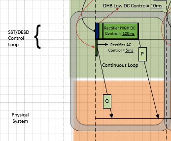
1. The vertical axis represents the following nodes 1. Group Management 2. State Collection 3. Load Balance 4. Demand/Member Node 5. DESD Control Loop 6. SST/DESD control loop and the 7.  Physical Layer.
   The horizontal axis represents timing in millisecond. The diagram represents a section where the DGI interacts with the physical devices.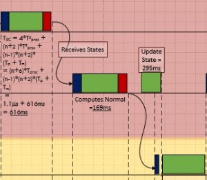
2. Different color schemes differentiate the type of process and time (for some instances). Each node is separated by different color. Green color represents the actual process being performed at particular node. Red colored box represents the message passing or calling procedure. The time for this equals 0.1µs (T).
   The dark blue box represents the time that a node takes to receive the call before starting the execution of request triggered (basically read the input). This is also equal to 0.1µs (T). White box represents timeout period.
3. The dashed lines separate the significant timeline changes. It separates the individual events at different nodes. It encloses empty slot that include the transmission delay (T) and propagation delay (T).
4. The arrows or pointers show that an event has been triggered. It is useful as both the source and destination is projected. In case of multiple triggers from a source different color distinguishes the destination. The processes which are sequenced to happen based on fixed time are represented without arrow.
5. Continuous Loops are represented in double border grey boxes, like the one shown at the SST/DESD control loop node.
6. Simultaneously occurring processes at same node are represented above and below the horizontal line assigned to the node. As not more than two processes occur at a single node, this scheme suffices.

Configuring Timings:

State Collection:
The state of the DGI consists of the states of each IEM, their software modules, and any messages in transit. The state collection module is invoked when a consistent state of the system is required (such as for fault diagnosis). The Chandy-Lamport state collection algorithm is used to collect a logically consistent state (one in which causality between actions is preserved). Modules submit requests to state collection, state collection runs those collections during it’s phase, and returns the collected state a message to the requesting module.

The Chandy-Lamport Algorithm:
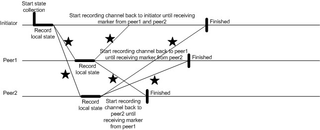
This algorithm is used to collect consistent states of all participants in a distributed system. A consistent global state is one corresponding to a consistent cut. A consistent cut is left closed under the causal precedence relation. In another words, if one event is belongs to a cut, and all events happened before this event also belong to the cut, then the cut is considered to be consistent. The algorithm works as follows:

• The initiator starts state collection by recording its own states and broadcasting a marker out to other peers. At the same time, the initiator starts recording messages from other peers until it receives the marker back from other peers.
• Upon receiving the marker for the first time, the peer records its own state, forwards the marker to others (include the initiator) and starts recording messages from other peers until it receives the marker back from other peers.

The following diagram illustrates the Chandy-Lamport algorithm working on three nodes. The initiator is the leader node chosen by Group Management module in DGI.

Group Management:
Group management provides consistent list of active DGI processes as well as identifies a primary process for initiating distributed algorithms. The group manager maintains the state of the system regarding the status of each IEM node, active, disabled, requesting entry, and requesting departure from the FREEDM system. In the event of IEM node failure or complete system failure and recovery, the group manager collaborates with its peer IEM nodes to reconstruct the FREEDM system using the Invitation Algorithm of Garcia-Molina. This algorithm provides a robust election procedure which allows for transient partitions. Transient partitions are formed when a faulty link inside a group of processes causes the group to divide temporarily. These transient partitions merge when the link becomes more reliable. In this fashion, IEM nodes become plug-and-play members of the FREEDM microgrid.

Group management will send all modules in the system a PeerList message when the list of active processes in the system changes. This message will also contain the identity of the leader process. Group management provides a static method for to aid processing this message. Group management can be configured to respect the topology of the physical network: it will not group two DGI unless a physical path exists between the two processes (as opposed to a cyber path).

Invitation Election Algorithm of Gracia-Molina:
The fundamentals of leader election are similar. Processes arrive at a consensus of a single peer that coordinates the group. Processes that fail are detected and removed from the group. The elected leader is responsible for making work assignments, identifying and merging with other coordinators when they are found, and maintaining an up-to-date list of peers. Group members monitor the group leader by periodically checking if the group leader is still alive by sending a message. If the leader fails to respond, the querying peers will enter a recovery state and operate alone until they can identify another coordinator. Therefore, a leader and each of the members maintain a set of currently reachable processes, a subset of all known processes in the system.

Using a leader election algorithm allows the FREEDM system to autonomously reconfigure 1 rapidly in the event of a failure. Cyber-components are tightly coupled with the physical components, and reaction to faults is not limited to faults originating in the cyber domain. Processes automatically react to crash-stop failures, network issues, and power system faults. The automatic reconfiguration allows processes to react immediately to issues, faster than a human operator, without relying on a central configuration point. The configuration a leader election supplies has two important characteristics. First, the configuration should allow the system to perform “work”. In the case of the DGI, this work is categorized as a grouping of DGI’s where, with the given configuration, any Power/Energy management algorithms running in that group can sucessfully coordinate resources. Secondly, the leader election algorithm should avoid configurations where the system does “bad” work. In these configurations, the algorithms may attempt to coordinate resources but physical or cyber network failures cause the work performed to contribute to the destabilization of the system. This destabilization can lead to physical faults such as voltage collapse and blackouts.

Execution occurs in a real-time partially synchronous environment. Processes synchronize their clocks and execute steps of the election algorithm at predefined intervals. Processes with clocks that are not sufficiently synchronized cannot form groups.

A state machine for the election portion of the election algorithm is shown in the figure below. In the normal state, the election algorithm regularly searches for other coordinators to join with. When another coordinator is identified, all other processes will yield to their future coordinator. The method of selecting which process becomes the coordinator of the new group differentiates the invitation election algorithm from other approaches. Coordinators and group members begin in the normal state. Coordinators identify each other by sending out “Are You Coordinator” (AYC) messages. Receiving processes respond in the positive if they are a coordinator, or the negative if they are not. In the invitation election algorithm, processes are assigned a priority based on their process ID. Using the list of coordinators determined with the AYC message, each coordinator determines its relative priority with respect to the other processes that sent the invites.

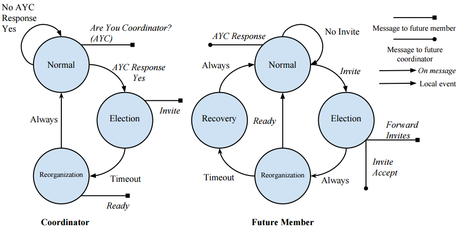
The coordinator with the highest priority is the first to send invites. When a coordinator sends invites, it switches to the election state. After a brief delay, if it appears that the highest priority coordinator did not send their invites, the next highest process will send their invites. A process will only accept an invitation if it is in the normal state. Coordinators that receive invites will forward the invite to its group members, if it accepts the invite. Those processes will accept the invite, sending a message to the process that originally sent the invitation. Once a timeout expires, the coordinator will send a “Ready” message with a list of peers to all processes that accepted the invite. The invited processes have timeouts for when they expect the “Ready” message to arrive. The coordinator, and any process that receives the “Ready” message will return to the normal state. If the “Ready” message does not arrive in time for a process, that process will enter the recovery state and reset to a group by itself.

Once a group is formed it must be maintained. To do this, processes occasionally exchange messages to verify the other is still reachable. This interaction is shown in the figure shown. Coordinators send “Are You Coordinator” messages to members of its group to check if the process has left the group. If a process does not respond to the AYC message or responds that they are a coordinator, they will be removed from the group. Group members send “Are You There” messages to the coordinator to verify they haven’t been removed from the group, and to ensure the coordinator is still alive. If the coordinator responds “no”, or fails to respond, the group member enters the recovery state where it resets to a group by itself.

As part of the DGI’s execution, the Group Management module runs before the start of execution for the Load Balancing and State Collection modules. Each time the algorithm is run the DGI attempts to discover new leaders to merge groups with and verifies the members of its group are still reachable.

Embedding Group State In Simulation:
The group state is by manipulating a “Logger” device on the FREEDM system. The value of device is updated each time the check or timeout procedure is called, that is, once at the beginning of the Group Management phase.

Data is stored in the device as a bit field. Because of the way data is passed to and from the RTDS and PSCAD the data is transported as a float, although the individual bits are unaffected by this process, it may be necessary to convert the float to an unsigned integer to be able to perform the bit fiddling needed to access the information.

This setup assumes that all DGI are aware of all other DGI in the system and that all the Group Management status tables are the same. This is reasonable because of the experiments we are currently running, and the fact that the container for the other DGIs in the system is a map. So when iterated, the items are returned in alpha numeric order.

C Broker:
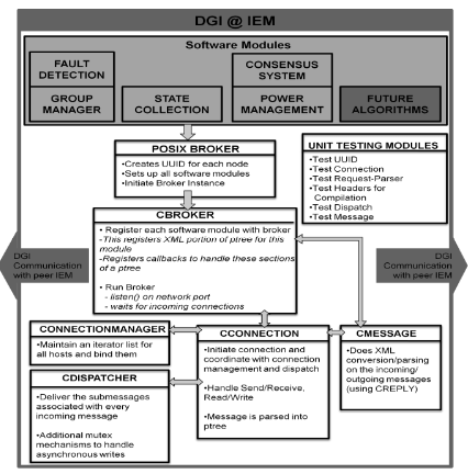
The DGI operating system architecture contains a ‘broker’ that integrates plug-in software modules. These include a group manager, state collection, and power management subsystem. In this way, changes in the configuration of the FREEDM system can be reflected in the power management and state collection modules. The following gives further details on these components.

The broker runs as a process that manages individual POSIX threads that invoke the CBroker class which instantiates each software module. A Connection Manager object maintains network connections with peer IEM nodes. This object tracks new and existing connections via the universally unique identifier (UUID) generated uniquely per-host when first executed. This UUID allows the Connection Manager to uniquely map connections to a specific peer node tracked in the group manager. This allows for nodes entering and leaving the network due to transient failures and initial activation of the IEM. The individual connections are managed by an event-triggered system that responds to message transmission, reception, and configurable timers. Each software module registers at runtime which types of messages it is interested in sending and receiving. The CDispatcher class parses incoming messages and dispatches them to the registered modules. Each message may contain more than one type of sub-message, allowing the modules managed by the broker to interact in a coordinated fashion. The incoming message is passed to the module message handlers in order that they were registered. The CDispatcher also provides the option for modules to handle outgoing messages, if needed. This is the case in the state collection module, as described below. In all cases, the CDispatcher provides a prioritized selection of messages and delivers them to their respective destinations, as directed.

The Scheduler:
The Scheduler performs real-time scheduling for execution of distributed algorithms. The real time scheduler uses a round robin approach. A module’s individual processing time is defined as it’s “Phase”. A round is composed of a GM (Group Management) Phase, an SC (State Collection) Phase and a LB (Load Balancing) Phase. Every DGI instance must have the same timing profile.

Message Processing:
When a message is received for processing, it will be taken into the CListener module where it is processed to determine if it should be accepted or rejected. If accepted, it is passed to the dispatcher which examines the contents to determine which modules if any should be given the message. The module responsible for receiving the message is immediately called and allowed to act on the message.

Phase Behavior:

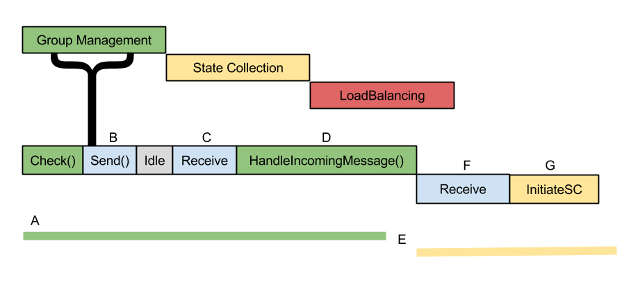
Phases proceed in a round robin fashion. However, there are some observations to make, for this implementation. Consider the diagram above.

1. The GM phase begins. It spends some time authoring messages for the check function, requests them to be sent and then idles. Send, which is handled by the broker operates outside of the module scheduler and begins work immediately.
2. Since group management has no work to do while waiting for replies, the system is idle.
3. Message(s) arrive. Since one of them is addressed to group management and it is currently in GM phase, the worker immediately fulfills the request.
4. Processing the message makes GM over-run its phase.
5. There is a “No-man’s” land where the group management task is completing work outside of its phase, but the scheduler is ready to switch phases to SC. Because phases are aligned in order to form groups, SC is penalized for by the overflow.
6. The scheduler has changed phases, but the broker does work on a received message before calling SC’s readied method. Note that the message is put into the ready queue for its intended process, so the message processing time is only spent by the Broker and communication stack
7. Finally, the SC module begins

Power Management (Load Balancing Module):
The power management module is a distributed application that schedules and balances the power load among IEM nodes. The power management algorithm negotiates via message passing with IEM nodes within the FREEDM system to control individual SSTs to add or subtract power to / from a shared power interconnection bus, thereby balancing the power on the microgrid in a way to meet the net demand/supply [4]. For this purpose, an extension of the concept of a locational marginal price (LMP) is employed. LMPs are used in transmission systems to provide a signal that is denominated in dollars per hour, and this signal is used to achieve certain objectives. In the transmission engineering application, the objectives are economic dispatch, alleviating line loads that are out of rating, and possibly insuring that the entire system is stable under the loss of a key transmission component (N-1 stable). In the distribution engineering application, a distribution class LMP is proposed, a D-LMP, to optimize energy storage, renewable energy controls, line loading management in the distribution network, and power usage. The D-LMP is formulated to render the FREEDM distribution system economically operable. D-LMP is carried out by the power management algorithm in reference

Distributed Load Balancing Algorithm:
The Load Balancing algorithm is published in “Distributed Load Balancing for FREEDM system” by Akella. The algorithm labels each process as being in Supply, Demand, or Neutral state and distributes that state to other processes in the group. Processes in the supply state have more generation and storage than load, neutral have equal generation and load, and demand processes have more load than generation. Each time the algorithm runs, a quantum of power is migrated from a supply process to a demand process. The amount that is migrated is a configurable but static value.

Overview of the Algorithm:
A majority of the work is controlled by the ‘LoadManage’ function. The function performs the following actions to complete the algorithm.

1. Schedule Next Round – The first thing the algorithm does is schedule the next time it will run. This will either be in the same phase or in the next phase. This is done to prevent the algorithm from running over its allotted execution time.
2. Read Devices – The state of the attached devices is read. This is done once per round so that the DGI can react to sudden changes in device state during the course of a load balance phase. Read devices measures the attached SST’s sum gateway value (which is the amount of power it is sending to other processes) and computes the difference between the power available and the attached load (generation + storage – load). This difference is the process’s “net generation”
3. Update State – This function uses the values measured after reading the devices to determine which load balancing state the DGI is in. If the amount of power the DGI is sending to other processes is less than the amount of net generation the SST has, and the DGI has sufficient net generation to send a migration to another process it is in the supply state. If the process is in a state where another quantum of power being drawn through the gateway would help it fulfill a deficit in net generation, the process is in a demand state. If neither of these conditions are met the process is in the normal state.
4. Load Table – This function prints the read device state and the state of the processes in the system to the screen.
5. At this point, the DGI checks to see if a “Logger” type device is attached. If the device is attached its “dgiEnable” value must be set to 1 for the DGI to actually perform a migration. If there is no device attached, the DGI will always attempt to perform a migration. This is useful for avoiding transients in some simulations. If the logger device is attached but the DGI is not enabled the DGI will write the gateway value it read in Read Devices back to the SST.
6. If the DGI process is in the demand state, the DGI sends an announcement to all other processes in its group inform them that it is in demand.
7. If the DGI process is in the supply state, it will check to see if it has received a message from state collection for the current phase. The collected state is used to set the initial value of a predicted SST gateway value that predicts how the SST’s real power injection will change in response to the DGI commands. This predicted value is used during the course of load balance instead of the measured SST real power injection since the power simulation may not respond immediately to DGI commands. If a message has not yet been received from state collection, then the supply node will do nothing for the current round.
8. After load balance receives the collected state message, the DGI will check the invariant. If the supply process determines the invariant hasn’t been violated, it will send a “Draft Request” message to all demand processes to offer them a migration. The DGI will then wait for responses to that message. Once this timeout expires the “Draft Standard” function will run.
9. On receipt of the Draft Request, the receiving process will note the sender is in a supply state and send a “Draft Age” message as a response. This message indicates the amount of demand the receiver has. This value is used by the sender (the supply process) to determine which processes have the greatest need.
10. On receipt of the “Draft Age” message, the supply node places the response in a table. When the timer expires and the “Draft Standard” function runs, the table is processed. Processes with an age of 0 are moved to the normal set. The process with the greatest age is selected. If that process’ age is greater than the size of a migration step, the supply process will send the selected demand process a “Draft Select” message. Additionally, the process will change its gateway value to send power to the selected demand process.
11. On receipt of the Draft Select message, the demand process will determine if it still need the offered power. If it does, it will send a Draft Accept message, and adjust its power levels to accept the incoming power. If it does not need the power it will respond with a Too Late message. If the Too Late message is received the supply node will roll back its half of the transaction with the demand node. If the Malicious flag is set, the DGI will drop the draft select message and not send the draft accept message.
12. On receipt of the Draft Accept message, the supply process notes that the transaction has been completed.
13. This process repeats a fixed number of times each round, determined by potential difference that DGI can accrue between the actual measurements and the predicted value while load balancing.

Limitations:

• The Load Balancing algorithm needs to be able to predict how the devices will react to its commands or the device will need to react instantaneously to its commands. If the device does not react sufficiently quickly enough, Load Balancing will repeatedly issue the same commands to the device and appear to not be working.
• This algorithm will move all power values to within one migration step of perfectly balanced. Since the migration step is currently a static value, the algorithm cannot perfectly balance the system. Additionally, there are many computations that include a migration step in order to prevent the DGIs from oscillating when they are near the perfect balance.

Fault Detection:
DGI is responsible for detecting internal software and hardware faults and receiving reports and sending commands to/from the Integrated Fault Management (IFM) system of FREEDM. Fault detection uses the state collection algorithm to obtain a consistent system state and employs correctness predicates to determine correct/faulty behavior. If a fault is detected, the consensus system and group manager are contacted to initiate reconfiguration around the failed component. In effect, this feature is automated restoration. The use of digital controllers in this application and the use of electronic circuit interruption make possible a substantial increase in reliability at networked distribution system buses.

Communications in DGI:
All communication between the DGI and physical devices is done through a set of classes called adapters. An adapter defines a communication protocol that the DGI uses to connect to real devices. The DGI can contain multiple adapters, and each adapter can use a different communication protocol. This allows, for instance, the DGI to talk to both a power simulation and real physical hardware at the same time. The DGI comes with multiple adapter types that can be used to interface with physical devices (either real or simulated). Configuration of the DGI depends on the type of adapter that is used. For almost all cases, an RTDS adapter is recommended. Despite its name, this adapter works with both RTDS and PSCAD, and has also been used to communicate with real hardware. Unless the user has extensive knowledge on the DGI, the RTDS adapter would be the best choice. The following sections document the two adapter types provided by the DGI team (RTDS and Plug and Play), as well as how to create a new adapter should neither option be viable.

1. RTDS Adapter:

The RTDS adapter was designed to allow the DGI to communicate with the FPGA connected to the RTDS rack at Florida State University. However, it has also become the default choice for connecting the DGI to a PSCAD simulation, and is a viable option when interfacing the DGI with real physical hardware. This is the adapter type recommended by the DGI development team for FREEDM. The term device server refers to the endpoint the DGI communicates with, while using the RTDS adapter. When using an RTDS simulation, the device server would be the FPGA server connected to the RTDS. When using PSCAD, the device server is a piece of code called the simulation server that runs on a linux computer. And when using real hardware, the device server refers to the controller attached to the physical device.

Communication Protocol:
The RTDS adapter uses TCP/IP to connect to a server with access to some set of physical devices. When the DGI runs using an RTDS adapter, it attempts to create a client socket connection to an endpoint specified in the adapter configuration file during startup. Once connected, it sends a periodic command packet to the server, and expects to receive a device state packet in return. The device server must be running and prepared to receive connections before the DGI starts when using an RTDS adapter. In addition, the DGI will always send its command packet before the device server responds with its state packet.

This communication protocol is very brittle. If the DGI loses connection to the server, it will not attempt to reconnect and after some time, the DGI process will terminate. In addition, if the DGI receives a malformed or unexpected packet from the server, it will terminate with an exception. Therefore, this protocol should only be used on a stable network.

The following diagram shows on round of message exchanges in the communication protocol. It assumes that there are three states produced by the devices, and one command produced by the DGI.

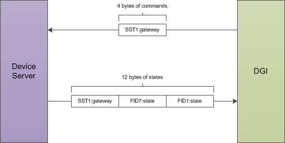
Both the command packet from the DGI and the state packet from the device server contain a stream of 4-byte floating point numbers. Other data formats such as boolean or string values cannot be used with the RTDS adapter; all the device states must be represented as floats. The command packet must contain every command for the devices attached to the server, while the state packet must contain every device state. It is not possible to send a subset of the commands, or to send the values for different commands at different times. If the DGI has not calculated the value of a particular command, it will send a special value of 10^8 to indicate a NULL command. The device server must recognize and ignore the value of 10^8 when parsing the command packet received from the DGI. Likewise, the device server can use the value of 10^8 for device states which are not yet available when communicating with the DGI.

2. Plug and Play Adapter:

The PNP Adapter allows the DGI to communicate with plug and play devices. Unlike the other adapter types, PNP adapters are created automatically and do not need to be specified in an adapter configuration file. However, by default, the plug and play behavior of the DGI is disabled.

Communication Protocol:
The plug and play protocol uses TCP/IP with the DGI listening for client connections from physical devices on a configurable port number. All packets in the protocol are written in ASCII and converted to floating point numbers within the DGI. An overview of both sides of the protocol is shown in the following state machine.

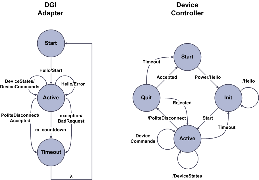
The protocol begins with both the DGI and the device controller in their respective start states. For the DGI, this state corresponds to sometime after the DGI has created its TCP/IP socket that listens for connections from devices. For the device, the start state represents when the device is powered off or disconnected. First, the device powers on and its controller sends the DGI a Hello message. The contents of this message tell the DGI which devices are connected to the controller, and the DGI uses the Hello message to construct a new plug and play adapter. If the new adapter is created without error, the DGI responds with a Start message and maintains the client socket for the duration of the protocol. A separate socket will be maintained for each concurrent plug and play connection to the DGI.

Once the plug and play adapter has been created, the DGI will remain in its active state until the device powers off, loses communication with the DGI, or causes an exception during the protocol. While in this state, the DGI expects the device to send it periodic DeviceStates messages which it will respond to with a corresponding DeviceCommands message. Unlike the RTDS adapter protocol, the DGI expects the device to send it the states before it issues commands. The plug and play connection is maintained by the DGI as long as it receives periodic DeviceStates messages from the device.

A device can gracefully disconnect from the DGI by sending a PoliteDisconnect message. However, if a device fails to send a DeviceStates message for a configurable timeout period, the DGI will close the socket connection and delete the plug and player adapter under the assumption the device has crashed or gone offline. As shown in the state machine, the DGI does not notify the device when it chooses to terminate the connection. If a device comes back online after the connection has been terminated, it must restart the protocol from the Hello message.